Bohr Model Simulation
February 22, 2026
Bohr Model Simulation: Hydrogen Atom & Quantum Mechanics
A computational physics project simulating the Bohr model of the hydrogen atom, including electron orbital dynamics, energy level calculations, emission spectra, and quantum wave functions.
Overview
This project implements a comprehensive simulation of the hydrogen atom based on Niels Bohr’s atomic model (1913). It combines classical orbital mechanics with quantum mechanical principles to visualize:
- Electron orbital motion in quantized energy levels
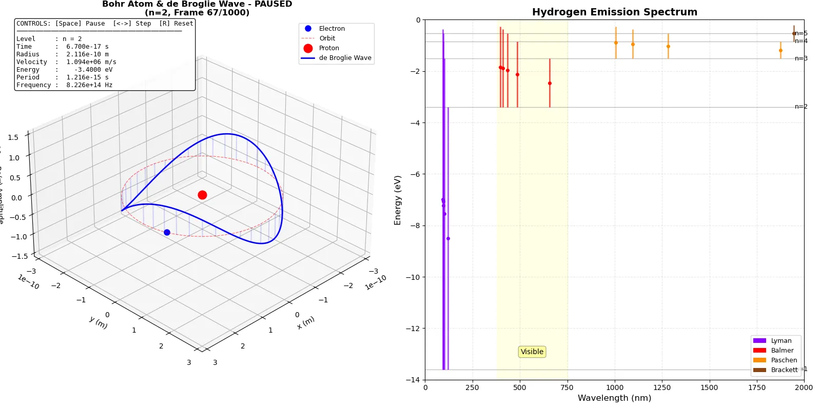
- Hydrogen emission spectrum (Lyman, Balmer, Paschen, Brackett series)
- de Broglie wave visualization on the electron orbit
- Quantum wavefunction evolution for a particle on a ring
Physical Background
The Hydrogen Atom
A hydrogen atom consists of:
- 1 Proton (nucleus, positive charge)
- 1 Electron (orbits the nucleus, negative charge)
The electron orbits the proton in quantized energy levels (not at arbitrary distances). These discrete orbital radii are called quantum states, labeled by the principal quantum number
Bohr Model Equations
1. Orbital Radius
The radius of the $n$-th orbit is given by:
where:
- m is the Bohr radius (ground state, )
- is the principal quantum number (1, 2, 3, …)
2. Electron Velocity
The orbital velocity in the -th state:
where:
- C (elementary charge)
- F/m (vacuum permittivity)
- J·s (Planck’s constant)
3. Energy Levels
The total energy of the electron in the -th state:
The negative sign indicates the electron is bound to the nucleus (ionization energy = 13.6 eV).
4. Photon Emission (Spectral Lines)
When an electron transitions from a higher energy level $n_2$ to a lower level $n_1$, it emits a photon with wavelength:
where is the Rydberg constant.
The photon energy is:
Project Structure
bohr_model/
├── main.c              # Main simulation entry point
├── bohr.h              # Header file with constants and function prototypes
├── utils.c             # Utility functions (radius, velocity, energy, wavelength)
├── specters.c          # Emission spectrum calculations (Lyman, Balmer, etc.)
├── wavefct.c           # Quantum wavefunction data (generated by simulation)
├── free_particle.c     # Free particle on a ring simulation
├── sim.py              # 3D animated visualization (Bohr orbit + de Broglie wave)
├── free_particle_sim.py # Wavefunction visualization for particle on ring
├── Makefile            # Build automation
├── data.csv            # Ground state orbital data (generated)
├── spectrum.csv        # Emission spectrum data (generated)
├── wavefct.csv         # Wavefunction evolution data (generated)
└── figue1.png          # Visualization screenshot
Console output (energy levels and spectrum):
=== BOHR MODEL - HYDROGEN ENERGY LEVELS ===

Level n | Radius (m)    | Velocity (m/s) | Energy (eV)
--------|---------------|----------------|-------------
   1    | 5.2900e-11    | 2.1877e+06     | -13.6000
   2    | 2.1160e-10    | 1.0939e+06     | -3.4000
   3    | 4.7610e-10    | 7.2923e+05     | -1.5111
   4    | 8.4640e-10    | 5.4693e+05     | -0.8500
   5    | 1.3225e-09    | 4.3754e+05     | -0.5440

=== HYDROGEN SPECTRUM (Selected Lines) ===

Balmer Series (Visible Light):
Transition | Wavelength (nm) | Energy (eV) | Color
-----------|-----------------|-------------|------------
  3 → 2    | 656.3           | 1.889       | Red (Hα)
  4 → 2    | 486.1           | 2.550       | Cyan (Hβ)
  5 → 2    | 434.0           | 2.856       | Blue (Hγ)
  6 → 2    | 410.2           | 3.022       | Violet (Hδ)
Generated files:
data.csv: Electron position vs. time for ground statespectrum.csv: All spectral line wavelengths and energieswavefct.csv: Quantum wavefunction evolution data
Key Results
1. Quantized Energy Levels
The simulation confirms that:
- Energy levels follow eV
- Ground state () has the lowest energy (-13.6 eV)
- Ionization (removing electron) requires 13.6 eV
2. Hydrogen Spectrum
- Accurately reproduces the Balmer series visible lines (observed in stellar spectra)
- UV Lyman series (seen in quasar absorption)
- IR Paschen/Brackett series (important in astrophysics)
3. de Broglie Wave-Particle Duality
The animation demonstrates that:
- Exactly wavelengths fit around the orbit circumference
- Wave and particle pictures are complementary
- Quantization arises from the standing wave condition:
Physical Constants Used
| Constant | Symbol | Value |
|---|---|---|
| Bohr radius | m | |
| Electron mass | kg | |
| Elementary charge | C | |
| Vacuum permittivity | F/m | |
| Planck constant | J·s | |
| Speed of light | m/s | |
| Rydberg constant | ||
| Ionization energy | - | 13.6 eV |
Limitations of the Bohr Model
While groundbreaking, the Bohr model has limitations:
- Only works accurately for hydrogen-like atoms (one electron)
- Cannot explain fine structure (spin-orbit coupling)
- Doesn’t predict intensity of spectral lines
- Replaced by Schrödinger equation (full quantum mechanics)
References
- N. Bohr, “On the Constitution of Atoms and Molecules”, Philosophical Magazine 26 (1913)
- A. Sommerfeld, “Atomic Structure and Spectral Lines” (1919)
- Griffiths, D.J., “Introduction to Quantum Mechanics”, 3rd ed. (2018)
- NIST Atomic Spectra Database
- Introduction to Quantum Mechanics